 When we think of prime numbers, the first thing that we tend to associate them with is randomness. Prime numbers are scattered all over the number line and there is no fixed formula that can tell you when the next one is going to occur. This has been used heavily by mathematicians and cryptographers to develop security systems for internet, banking, communication, and so on. Coming to the topic at hand, we are going to talk about prime divisors of a given number. Prime divisors of a number are divisors of that number that happen to be prime numbers. Big surprise, right? Alright, what’s so interesting about them?
Understanding prime divisors
Let’s consider an example. If we factorize the number 12, you will see that it can be written as 2 x 2 x 3. As we can see, 12 has two unique prime divisors i.e. 2 and 3. If you consider 60, it can be written as 2 x 2 x 3 x 5. In this case, it has three prime divisors i.e. 2, 3, and 5. Let’s build a function, ω(n), that will count the number of unique prime divisors for a given number. For example, ω(60) will be equal to 3, because 60 has 3 unique prime divisors. Basically, any number can be written as a product of prime numbers. That’s an established fact! If you take a number and keep breaking it down, you will eventually reach a stage where all the factors are prime. Now, if we compute the value of ω(n) for a lot of numbers, we will see that something interesting emerges.
What’s that interesting thing?
To understand the interesting thing, we need to visualize it. Alex Beckwith gives a nice visual summary of this function his tutorial. If you get a chance, you should check it out. Let’s look at the graph here:
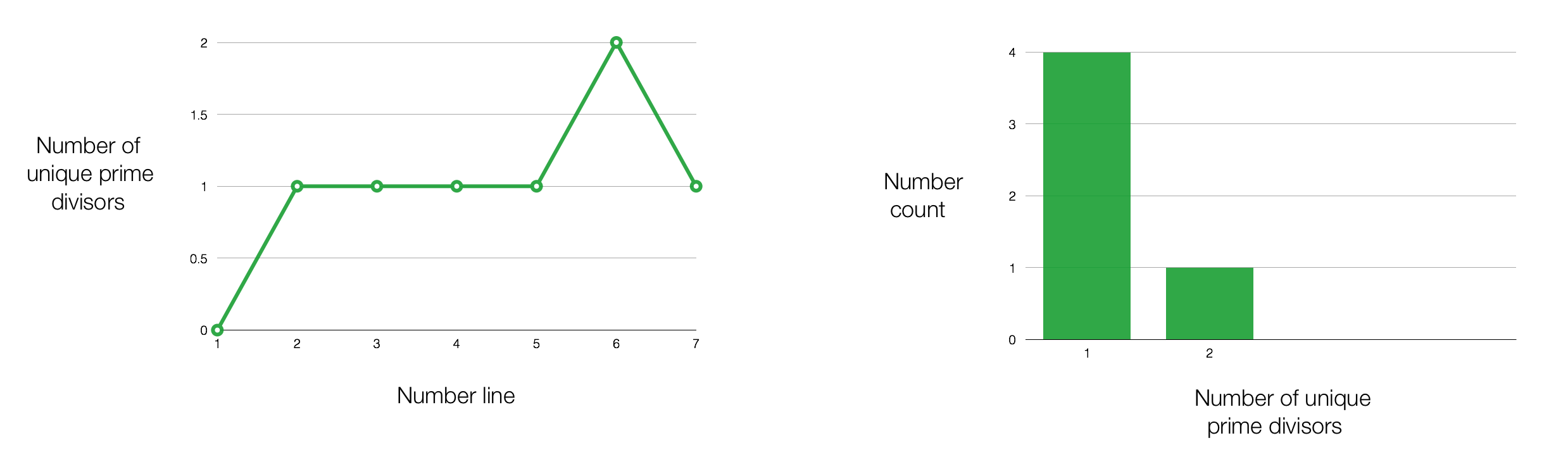
In the graph on the left, the X axis is the number line and Y axis represents the number of unique prime divisors of each number. Now let’s change things up a bit in the graph on the right. In this graph, we consider a particular number, say ‘7’. For this number, we plot the number of unique prime divisors on the X axis and the number of positive integers that have these many prime divisors. For example, the value at x=1 is 4. It means that there are 4 numbers between 1 and 7 that have only 1 unique prime divisor. We also have the value 1 at x=2, which means that there is only 1 number that has two prime divisors. Simple enough, right? Okay let’s proceed.
What are we looking at?
 In Beckwith’s tutorial, he plots an interesting graph by considering various different numbers as shown in the figure to the left. Just so we are all on the same page, let’s understand what this means. Let’s consider the graph on the second row in the third column in the figure. Here, we take the number ‘1000’ and then plot the graph using our second method (prime divisors on the X axis). The interesting thing is that if you keep doing this for bigger and bigger numbers, the curve starts to look like a Gaussian! The Gaussian curve looks like this:
 If you are not familiar with Gaussians, you should read the wiki article. A Gaussian curve is used to describe the distribution of data points. It is probably one of the most famous curves in all of mathematics. It’s also heavily used in physics, chemistry, cryptography, computer vision, machine learning, and so on.
Okay so it’s a Gaussian! What’s the big deal?
The interesting thing here is that there is a pattern that governs the number of prime divisors. Any “pattern” that can be associated with primes becomes instantly interesting because primes just refuse to fit into any patterns. If we can find some pattern, then it can lead to a lasting impact in number theory, and hence modern cryptography. That’s why we need to understand this!
As we can see here, as the numbers get larger, the number of prime divisors of those numbers start to fit into beautiful Gaussian curves. Not only that, we can also compute the mean and variance of that Gaussian curve. Both mean and variance values are equal to log(log N) where N is the number under consideration. The “mean” is basically the point where the Gaussian curve “peaks” and the variance refers to the “width” of the Gaussian curve. Low variance indicates a narrow Gaussian curve! The fact that the prime divisors fit into a Gaussian curve is formalized into a theorem, and this theorem is known as Erdos-Kac theorem.
———————————————————————————————————
