How To Compute Confidence Measure For SVM Classifiers

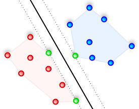
Support Vector Machines are machine learning models that are used to classify data. Let’s say you want to build a system that can automatically identify if the input image contains a given object. For ease of understanding, let’s limit the discussion to three different types of objects i.e. chair, laptop, and refrigerator. To build this, we need to collect images of chairs, laptops, and refrigerators so that our system can “learn” what these objects look like. Once it learns that, it can tell us whether an unknown image contains a chair or a laptop or a refrigerator. SVMs are great at this task! Even though it can predict the output, wouldn’t it be nice if we knew how confident it is about the prediction? This would really help us in designing a robust system. So how do we compute these confidence measures?  

Where do we start?

This discussion is specifically related to scikit-learn. It is a famous Python library that’s used extensively to build machine learning systems. It offers a variety of algorithms and tools that are useful to develop these systems. Let’s quickly build an SVM to get started:

>>> import numpy as np
>>> from sklearn.svm import SVC
>>> X = np.array([[2, 1], [6, 2], [5, 3], [3, 0], [5, 4], [1, 1]])
>>> y = np.array([0, 1, 1, 0, 1, 0])
>>> classifier = SVC(kernel='linear')   # Initialize the SVM
>>> classifier.fit(X, y)                # Train the SVM

Let’s visualize the datapoints:

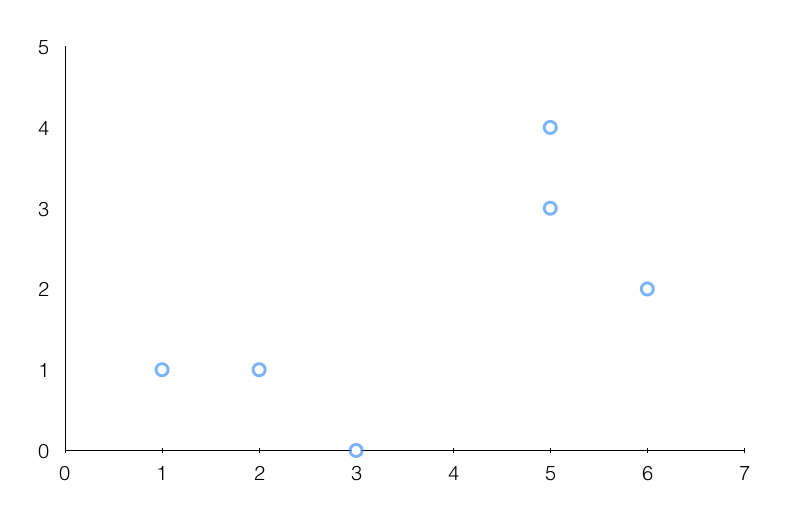
We can clearly see that the datapoints can be divided into two groups. Now, let’s say there is a new datapoint like [1, 3] and we want to predict which class it belongs to. We just need to run the following command:

>>> classifier.predict([1, 3])
array([0])

It says that this datapoint belongs to class 0. We can look at the graph and visually confirm that this is infact correct.

How far is it from the boundary?

Although we know which class it belongs to, we don’t know how far it is from the boundary. Let’s consider two points, say [4, 2] and [1, 0]. If you plot these points on the graph, we can confidently say that [1, 0] belongs to class 0. But [4, 2] lies right on the boundary and we are not so sure where it’s going to go. So we need a way to quantify this! To do that, we have a function called “decision_function” that computes the signed distance of a point from the boundary. A negative value would indicate class 0 and a positive value would indicate class 1. Also, a value close to 0 would indicate that the point is close to the boundary.

>>> classifier.decision_function([2, 1])
array([-1.00036982])

It is very confident that [2, 1] belongs to class 0. Let’s see what it says about [4, 2]:

>>> classifier.decision_function([4, 2])
array([ 0.20007396])

It says it belongs to class 1 but based on the output value, we can see that it’s close to the boundary.

Is this the same as confidence measure?

Not exactly! In the above example, “decision_function” computes the distance from the boundary but it’s not the same as computing the probability that a given datapoint belongs to a particular class. To do that, we need to use “predict_proba”. This method computes the probability that a given datapoint belongs to a particular class using Platt scaling. You can check out the original paper by Platt here. Basically, Platt scaling computes the probabilities using the following method:

P(class/input) = 1 / (1 + exp(A * f(input) + B))

Here, P(class/input) is the probability that “input” belongs to “class” and f(input) is the signed distance of the input datapoint from the boundary, which is basically the output of “decision_function”. We need to train the SVM as usual and then optimize the parameters A and B. The value of P(class/input) will always be between 0 and 1. Bear in mind that the training method would be slightly different if we want to use Platt scaling. We need to train a probability model on top of our SVM. Also, to avoid overfitting, it uses n-fold cross validation. So this is a lot more expensive than training a non-probabilistic SVM (like we did earlier). Let’s see how to do it:

>>> classifier_conf = SVC(kernel='linear', probability=True)
>>> classifier_conf.fit(X, y)
>>> classifier_conf.predict_proba([1, 3])
array([[ 0.67902586, 0.32097414]])

It is 67.9% sure that this point belongs to class 0 and 32.1% sure that it belongs to class 1. Let’s see what it says about [4, 2]:

>>> classifier_conf.predict_proba([4,2])
array([[ 0.43254616, 0.56745384]])

It is 43.25% sure that it belongs to class 0 and 56.74% sure that it belongs to class 1. As we can see, the decision is not very clear, which seems fair given the fact that this point is close to the boundary. Looks like we are all set!

————————–————————–—————————————————–