 In the field of computer vision, we often come across situations where we need to recognize the shapes of different objects. Not only that, we also need our machines to understand the shapes so that we can identify them even if we encounter them in different forms. Humans are really good at these things. We somehow make a mental note about these shapes and create a mapping in our brain. But if somebody asks you to write a formula or a function to identify it, we cannot come up with a precise set of rules. In fact, the whole field of computer vision is based on chasing this hold grail. In this blog post, we will discuss a particular model which is used to identify different shapes.
What exactly is it?
The Point Distribution Model (PDM) is a shape description technique that is used in locating new instances of shapes in images. It is also referred to as Statistical Shape Model. It basically tries to “understand” the shape, as opposed to just building a rigid model. It is very useful for describing features that have well understood general shape, but which cannot be easily described by a rigid model. The PDM has seen enormous application in a short period of time. PDM basically represents the mean geometry of a shape, along with statistical modes of geometric variation inferred from a training set of shapes.
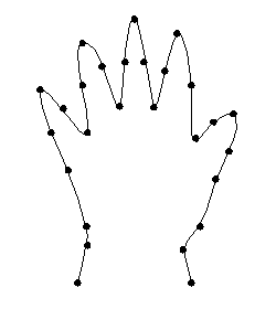 It is formulated by combining local edge feature detection and a model based approach. This gives a fast and simple method of representing an object and how its structure can deform. Read the last part of the previous sentence carefully! This is what differentiates it from other models. The representation includes the way in which the structure can deform. We need to understand that PDM relies on landmark points. A landmark is basically an prominent point on a given locus for every shape instance across the training set. For example, as seen from the picture here, the tip of the index finger in a training set of 2D hand-outlines can be designated as a landmark point. Principal component analysis (PCA) is a relevant tool for studying correlations of movement between groups of landmarks among the training set population. Typically, it might detect that all the landmarks located along the same finger move exactly together across the training set examples showing different finger spacing for a flat-posed hands collection.
How does it work?
Given a set of examples of a shape, we can build a statistical shape model. Each shape in the training set is represented by a set of ‘n’ labeled landmark points, which must be consistent from one shape to the next. For instance, let’s say we trying to locate a hand. If we track a unique set of points, the kth point may always correspond to the tip of the thumb. Given a set of such labeled training examples, we align them into a common co-ordinate frame. This translates, rotates and scales each training shape so as to minimize the sum of squared distances to the mean of the set.
 The PDM approach assumes the existence of a set of M examples. These M examples comprise the training set. As is true with any machine learning algorithm, a good training set can make a huge difference. Now, from this training set, we derive a statistical description of the shape and its variation. In our hand example, we take this to mean some number of instances of the shape represented by a boundary, which is actually a sequence of pixel co-ordinates. In addition, ‘N’ landmark points are selected on each boundary. These points are chosen to correspond to a feature of the underlying object.
It is necessary first to align all the training shapes in an approximate sense. This is done by selecting for each example a suitable translation, scaling and rotation to ensure that they all correspond as closely as possible. The transformations are chosen to reduce the difference between an aligned shape and a `mean’ shape derived from the whole set.
What’s the advantage?
A strength of this approach is that it permits plausible shapes to be fitted to new data.
Due to the properties of principal component analysis, eigenvectors are mutually orthogonal. This means that they can form a basis of the training set cloud in the shape space. The shape at the origin in this space represents the mean shape. Also, PCA is a traditional way of fitting a closed ellipsoid to a Gaussian cloud of points, which suggests the concept of bounded variation. The idea behind PDM is that eigenvectors can be linearly combined to create infinite new shape instances that will “look like” the one in the training set. The coefficients are bounded like the values of the corresponding eigenvalues, so as to ensure the generated n-dimensional dot will remain into the hyper-ellipsoid in the allowable shape domain. That was a bit of computer vision jargon! If you didn’t understand it, you should read up a bit on PCA. It’s a very important concept and it’s widely used in many fields. If you are ever in a situation where you have to build a good shape detection algorithm, you should definitely check out point distribution models.
————————————————————————————————-

Reblogged this on Coconuts Health Blog.