Image Classification Using Fisher Vectors

This is a continuation of my previous blog post on image classification and the bag of words (BoW) model. If you already know how BoW works, then you will feel right at home. If you need a refresher, you can read the blog post here. In our previous post, we discussed how BoW works, and how we construct the codebook. An interesting thing to note is that we don’t consider how things are ordered as such. A given image is treated as a combination of codewords regardless of where they are located with respect to each other. If we want to improve the performance of BoW, we can definitely increase the size of the vocabulary. If we have more codewords, we can describe a given image better. But what if we don’t want to do that? Is there a more efficient method that can be used?  

What are the shortcomings of BoW?

Before we go ahead and discuss other methods, let’s understand why we need them in the first place. According to our current method, we represent a given image with a histogram. But it is not clear as to why such a histogram representation should be optimal for our classification problem in the first place. When we do vector quantization, we don’t consider how far a given feature is from the codeword. Let’s consider the example of categorization of the human population based on cities. We choose a representative city for a geographical area and say that all the people in that area belong to that city. This means that a town which is very close to the city gets the same weight as the town that’s far away but still within the same geographical area. Even though we are quantizing, it would be nice to account for this kind of distribution. This is one of the problems with BoW model. It doesn’t encode any local statistic!

We want our new method to encode this kind of distribution effectively and take it into account when we classify images. In BoW model, we don’t consider how the features are ordered with respect to each either. Also, the descriptor quantization is a lossy process. This is equivalent to losing the information about the distances of those two towns from the city. The performance depends on the quantization level. At the same time, we should be careful about how much information we end up adding. In recent years, the computational cost has become an important issue in image classification.

VLAD the Impaler

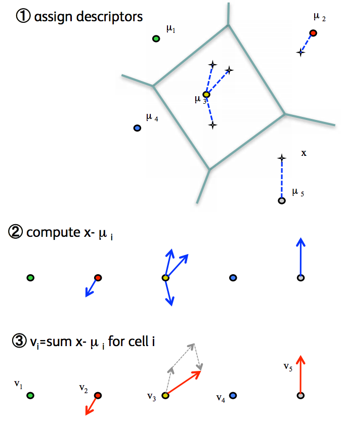Before we proceed, did you get the joke? If not, go ahead and read this article on Vlad the Impaler. He was a ruthless Romanian ruler who impaled prisoners of war in a gory way. But what we are about to discuss has nothing to do with him. In our case, VLAD stands for Vector of Linearly Aggregated Descriptors. This is another model that we use for image classification. All the steps here are very similar to what we did in BoW, including generating the codebook. But once we have the codebook, the method in which we encode the stats is different. Instead of just storing the class to which a particular feature belongs to, we compute the distance to the nearest centroid and store it. This is called first order statistic. As you can in the figure here, the point near µ₂ is closer to the centroid than the point near µ₅. In the BoW model, this is not accounted for. Hence we end up losing this information. In the VLAD model, this information is stored for each class and is used as a measure.

So as we can see here, we are basically storing more information about the distribution of these feature points. This makes the model more discriminative, which means that we can classify the images better. Now that we have added a first order statistic, one might wonder if we can go any higher. If adding an order of statistic makes it better, can we add one more to make it even better? When we compute these feature vectors and assign a codeword, we are speculating that everything went right. Sometimes things don’t go according to plan, and we need a way to measure the confidence with which we are doing this. So can we do it in a probabilistic way to make it more flexible? Well, yes! That’s where the Fisher Vectors come into picture.

Fisher Vectors

As we saw earlier with VLAD, we want to make the model more flexible. Fisher Vector (FV) are named after Sir Ronald Fisher, an English mathematician who made significant contributions to the field of statistics. FV is basically an image representation obtained by pooling local image features, and it is used as a global image descriptor in image classification. Wait a minute, isn’t that what VLAD does too? Yes, that’s true! But there are a couple of important differences. First of all, the VLAD model does not store second-order information about the features, where as FV does. Secondly, VLAD typically use K-Means to generate the feature vocabulary, where as FV uses Gaussian Mixture Models (GMMs) to do the same. So instead of constructing a hard coded codebook, we generate a probabilistic visual vocabulary. This allows us to be more flexible. This is a very important feature which helps in improving the performance.

Why GMMs?

You must be wondering why we use GMMs here. Okay, let’s talk a little bit about it. GMMs are used whenever we have subpopulations in our data. For example, let’s say that we have a some data and we know that it can be divided into 5 classes. This indicates the presence of 5 subpopulations in our data, and hence we can use GMM to model this. If you need a refresher on GMMs, I have discussed it in detail here.

If we use a probability density function, like GMM, we can compute the gradient of the log likelihood with respect to the parameters in the image. Now what on earth is this “log likelihood”? In statistics, we have something called likelihood functions. These are functions of the parameters of a particular statistical model. Whenever we have a lot of data, we want to estimate to underlying parameters. So the likelihood function tells us how likely we are to observe a set of parameters given that we have observed a bunch of these outcomes. For mathematically convenience, we take the natural logarithm of this function and call it log-likelihood. Coming back to GMMs, we use them in the construction of FVs. The FV is obtained by concatenating these partial derivates and it describes in which direction the parameters of the model should be modified to best fit the data. The good thing about this is that it gives better performance than BoW model.

FV vs BoW

The FV representation has many advantages over BoW. BoW doesn’t give us flexibility as to how we can define our kernel. Using FV, we can have a more general way to define a kernel from a generative process of the data. By “generative process”, we mean that we take into account how the data is generated, as opposed to just defining a fixed kernel. If you are not sure what a kernel is, this wiki article might be useful. It has been proven that BoW is a particular case of the FV where the gradient computation is restricted to the mixture weight parameters of the GMM.

Another advantage of FV is that it can be computed from much smaller vocabularies, and therefore at a lower computational cost. As we discussed earlier, the size of the vocabulary was one of the concerns of the BoW model. Another advantage of FV is that it performs well even with simple linear classifiers. Now how is that an advantage? If you recall, once you extract a feature, we need a classifier to separate things into different classes. Now, if the things are not clearly separated, we need a higher level model which will come up with curvy and complex boundaries between classes. This tends to add unwanted complexity! If we have a good model, a simple linear classifier will work just fine. This is what FV gives us. A significant benefit of linear classifiers is that they are very efficient to learn and easy to evaluate.

—————————————————————–————-——————-